📁 Chapter 2: Feedforward Neural Network (FNN) Summary

1. Overview of Feedforward Neural Networks (FNN)

FNN = Feedforward Neural Network (also called Fully Connected Neural Network).
Most FNNs adopt a fully connected architecture, so the two terms are often used interchangeably.
It is another name for the Multilayer Perceptron (MLP), the most fundamental form of an artificial neural network.
Universal Approximation Theorem:
With a sufficient number of hidden neurons and an appropriate activation function, an FNN can approximate any n-dimensional continuous function to an arbitrary degree of accuracy.

2. Structure and Design of FNN

An FNN has unidirectional data flow — signals move only forward.
Each neuron performs weighted summation → activation function.
Importantly, it assumes independence among data points (no recurrent connections).

2.1 Layer Structure

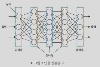
Input layer: receives external data
Hidden layer(s): extracts features
Output layer: produces predictions or classifications

Usually there is one input and one output layer;
the number of hidden layers varies depending on task complexity.

2.2 Fully Connected (FC) Layers

Every neuron in one layer is connected to every neuron in the previous layer.
Even with the same input, different neurons extract different features — more neurons allow richer representation.
Weighted summation: assigns greater weights to important features.
$$ z = \sum_i w_i x_i + b $$
Activation function: introduces nonlinearity, essential for learning complex patterns (e.g., XOR).

2.3 ReLU (Rectified Linear Unit)

$$x > 0 \Rightarrow x,\quad x \le 0 \Rightarrow 0$$
Computationally efficient and stabilizes training.
Neural networks must be differentiable (or piecewise differentiable) to allow backpropagation.

2.4 Universal Approximation and Network Depth

Even a 2-layer FNN can approximate continuous functions with enough hidden neurons.
However, increasing neurons arbitrarily leads to overfitting →
stacking deeper layers can achieve the same performance with fewer neurons.

2.5 Design Checklist

Input shape
Output shape / activation function
Hidden-layer activation function
Network size (depth & width)

3. Classification vs. Regression

Classification: predicts a category (class).
Regression: predicts a continuous value.

Classification can be viewed as a discriminant function (decision boundary) or a probabilistic model (predicting class probabilities).

4. Binary Classification Model

Binary classification models predict a Bernoulli distribution.

Output activation: Sigmoid
$$\sigma(z) = \frac{1}{1 + e^{-z}}$$
Loss function: Binary Cross-Entropy, which pairs naturally with the sigmoid output.

5. Multi-class Classification Model

Multi-class classification predicts a categorical (multinomial) distribution.

Output activation: Softmax
$\mathrm{softmax}(z)_k = \frac{e^{z_k}}{\sum_j e^{z_j}}$
Loss function: Categorical Cross-Entropy

Note: Binary classification can also be expressed as a 2-dimensional softmax,
but it’s typically simplified to a 1-dimensional sigmoid model.

6. Regression Model

Regression often assumes observation noise follows a Gaussian distribution.
The model usually predicts the mean ( \mu = y(x) ) only (variance is treated as constant).
Output activation: Identity function.

7. Input Layer

If the input is an n-dimensional vector, the input layer should have n neurons.
Example: a 28×28 image is flattened into a 784-dimensional input vector.

8. Summary of Activation Functions

8.1 Sigmoid Family

Pros: differentiable everywhere, squashes values into [0, 1].
Cons: exponential computation cost, gradient saturation/vanishing,
outputs are positive → optimization path may oscillate.

8.2 Hyperbolic Tangent (tanh)

Range [-1, 1], reducing oscillation in optimization.
Still suffers from exponential computation and saturation problems.

8.3 ReLU Family

ReLU: fast, robust to saturation/vanishing.
Leaky ReLU / PReLU: assigns small slope in negative region to mitigate “dead ReLU.”
ELU: exponential negative region — stable even for large negative inputs.
Maxout: neuron output = max of several linear functions → activation is learned.
Swish (SiLU): (x \cdot \sigma(x)); modern nonlinearity with strong empirical performance.

9. Network Size (Width & Depth)

Width: number of neurons per layer
Depth: number of layers
Search strategies: Random Search is generally more efficient than exhaustive Grid Search.
Modern approaches include Neural Architecture Search (NAS) for automated structure optimization.

9.1 Scaling Strategy

As demonstrated by EfficientNet, jointly scaling width, depth, and input resolution —
called Compound Scaling — yields more efficient performance improvements.

Download PDF